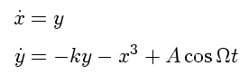
日前從圖書館借了一本書 From Calculus to Chaos ,這本書主要是在介紹 動態系統 的一些特性,附了很多例子, 其中第4章有介紹如何用 Runge Kutta 方法來求得微分方程的數值解, 方法是出乎我意料之外的簡單,於是找了一個例子來練習,考慮下面的 Duffing equation
為了用 Runge Kutta 方法,要先把上式改寫為
Duffing equation 是二階非線性時變微分方程,二階是因為 \ddot{x}, 非線性是因為 x^3,而時變是因為 cos \Omega t。我是用 Python 來寫,用 Matplotlib 來做繪圖的工作, 注意在安裝 Matplotlib 之前需先安裝 Numpy。
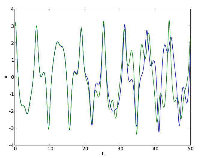
所使用的參數是 k=0.05, A=7.5, \Omega=1, 上圖的曲線是 x 對 t 做圖,兩條曲線的初始條件 (x, y) 分別為 (3.003, 3) 跟 (3, 3), 即兩個初始條件的差別只在第一個元素,而且只差了 0.003,可是從上圖可知大概在 20 秒之後, 兩條曲線開始有明顯的差異,這就是混沌系統 ( chaotic system ) 的特性之一, 系統對於初始條件的變化非常敏感,初始條件的微小變動會造成系統動態的巨大改變。 程式碼如下: (我是用 GeSHi 做 syntax highlight,程式碼在 chaos.py )
from math import cos
k = 0.05
Omega = 1
A = 7.5
def f(t, state):
[x, d_x] = state
y = d_x
d_y = -k * d_x - x*x*x + A*cos(Omega*t)
return array([y, d_y])
def Runge_Kutta(a, b, h, initial):
z = []
state = initial
hh = h/2
for t in arange(a, b+h, h):
z.append(state[0])
k1 = f(t, state)
k2 = f(t+hh, state+hh*k1)
k3 = f(t+hh, state+hh*k2)
k4 = f(t+h, state+h*k3)
state += h/6 * (k1 + 2*k2 + 2*k3 + k4)
return z
a = 0
b = 50
h = 0.01
z = Runge_Kutta(a, b, h, [3, 3])
y = Runge_Kutta(a, b, h, [3.003, 3])
t = [i for i in arange(a, b+h, h)]
plot(t, z, t, y)
xlabel('t')
ylabel('x')
show()
程式碼很簡單,我只介紹兩個 Numpy 提供的函式,分別是 arange() 跟 array(), Python 內建 range() 的參數型態只能是整數,Numpy 提供的 arange() 則允許參數型態是浮點。 學過線性代數都知道,向量空間中最基本的兩個運算分別是純量乘法跟向量加法,比如
    2 [1, 2, 3] = [2, 4, 6]
    [1, 2, 3] + [1, 0, 1] = [2, 2, 4]
可是 Python 內建的 list 型態,並沒提供這兩種運算,但是如果是用 array() 所宣告的型態, 則可直接使用這兩種運算。 有了 Numpy 提供的 arange() 跟 array (),程式碼是不是看起來就跟 維基百科 所列的演算法相差無幾呢?這就是 Python 程式語言的迷人之處, 趕快來學 Python 吧!
註:我是在 Yukuan's Blog 發現 Matplotlib 這個好用的 Python 函式庫。
